
多标签分类问题
Difference between multi-class classification & multi-label classification is that in multi-class problems the classes are mutually exclusive, whereas for multi-label problems each label represents a different classification task, but
the tasks are somehow related.
multi-class classificationmakes the assumption that each sample is assigned to one and only one label: a fruit can be either an apple or a pear but not both at the same time. Whereas, an instance ofmulti-label classificationcan be that a text might be about any of religion, politics, finance or education at the same time or none of these
Problem Definition & Evaluation Metrics
Problem Definition:
- conformation classification is a multi-label classification problem with a highly imbalanced dataset.
- We’re challenged to build a
multi-labeld modelthat’s capable of detecting different types of conformation like cidi, cido, codi, codo, w. W e need to create a model whichpredicts a probability of each type of conformation for each ligand.
Evaluation Metrics:
Note: Initially evaluation metric in the model task challenge was Log-Loss, which was later changed to AUC. But in this post we throw light on other evaluation metrics as well.
- The evaluation measures for
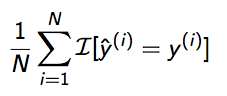
single-labelare usually different than for multi-label. Here in single-label classfication we use simple metrics such as precision, recall, accuracy, etc,. Say, in single-label classification,accuracyis just:
- In
multi-label classification, a misclassification is no longer a hard wrong or right. A prediction containing a subset of the actual classes should be considered better than a prediction that contains none of them, i.e.,predicting two of the three labels correctly this is better than predicting no labels at all.
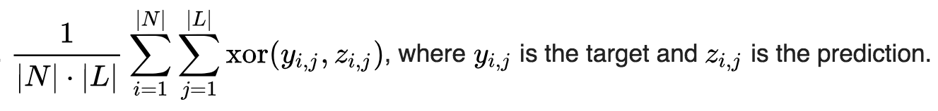
Hamming-Loss (Example based measure):
- In simplest of terms, Hamming-Loss is the fraction of labels that are incorrectly predicted,
i.e.,
the fraction of the wrong labels to the total number of labels.
N: number of samples
L: number of labels
number of wrong / N * L
Averaging
Macro-averaging
宏平均(Macro-averaging)是指所有类别的每一个统计指标值的算数平均值,也就是宏精确率(Macro-Precision),宏召回率(Macro-Recall),宏F值(Macro-F Score),其计算公式如下:
[公式]
[公式]
[公式]
Micro-averaging
微平均(Micro-averaging)是对数据集中的每一个示例不分类别进行统计建立全局混淆矩阵,然后计算相应的指标。其计算公式如下:
[公式]
[公式]
[公式]
Macro-averaging与Micro-averaging的不同之处在于:Macro-averaging赋予每个类相同的权重,然而Micro-averaging赋予每个样本决策相同的权重。因为从 值的计算公式可以看出,它忽略了那些被分类器正确判定为负类的那些样本,它的大小主要由被分类器正确判定为正类的那些样本决定的,在微平均评估指标中,样本数多的类别主导着样本数少的类。
Exact Match Ratio (Subset accuracy):
- It is the
most strictmetric, indicating the percentage of samples that have all their labels classified correctly.
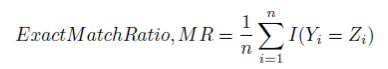
- The disadvantage of this measure is that multi-class classification problems
have a chance of being partially correct,but here we ignore those partially correct matches. - There is a function in _scikit-learn _which implements subset accuracy, called as accuracy_score.
Note: We will be using accuracy_score function to evaluate all our models in this project.
Multi-Label Classification Techniques:
Most traditional learning algorithms are developed for single-label classification problems. Therefore a lot of approaches in the literature
transform the multi-label problem into multiple single-label problems, so that the existing single-label algorithms can be used.
1. OneVsRest
- Traditional two-class and multi-class problems can both be cast into multi-label ones by restricting each instance to have only one label. On the other hand,
the generality of multi-label problems inevitably makes it more difficult to learn. An intuitive approach to solving multi-label problem is to decompose it into multiple independent binary classification problems (one per category) - In an “one-to-rest” strategy, one could
build multiple independent classifiersand, for an unseen instance, choose the class for which the confidence is maximized. - The
main assumptionhere is that thelabels are _mutually exclusive_. You do not consider any underlying correlation between the classes in this method. - For instance, it is more like asking simple questions, say, “is the comment toxic or not”, “is the comment threatening or not?”, etc. Also there might be an extensive case of overfitting here, since most of the comments are unlabeled, i,e., most of the comments are clean comments.
2. Binary Relevance
- In this case an ensemble of single-label binary classifiers is trained, one for each class.
Each classifier predicts either the membership or the non-membership of one class.The union of all classes that were predicted is taken as the multi-label output.This approach is popular because it is easy to implement, however it also ignores the possible correlations between class labels. - In other words,
if there’s _q_ labels, the binary relevance method create _q_new data sets from the images, one for each label and train single-label classifiers on each new data set. One classifier may answer yes/no to the question “does it contain trees?”, thus the “binary” in “binary relevance”. This is a simple approach but does not work well when there’s dependencies between the labels. - OneVsRest & Binary Relevance seem very much alike. If multiple classifiers in OneVsRest answer “yes” then you are back to the binary relevance scenario.
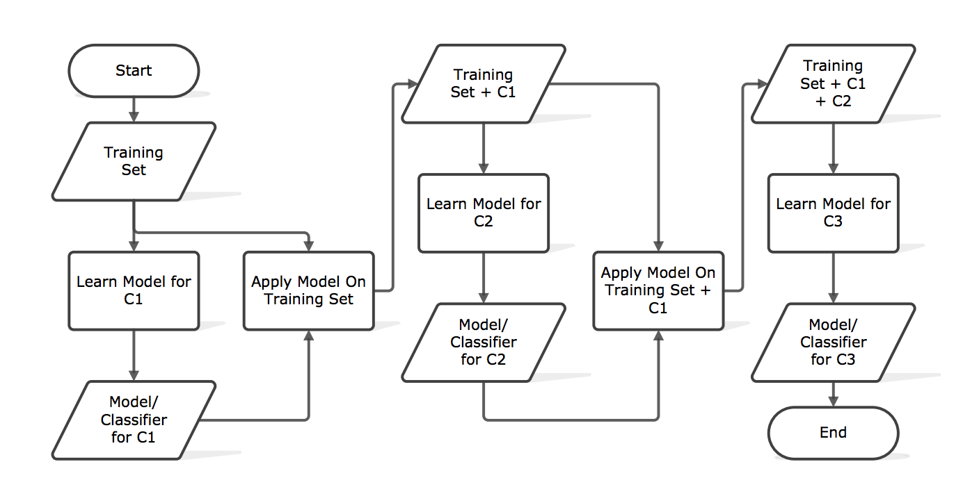
3. Classifier Chains
- A chain of binary classifiers C0, C1, . . . , Cn is constructed, where a classifier Ci uses the predictions of all the classifier Cj , where j < i. This way the method, also called classifier chains (CC), can take into account label correlations.
- The total number of classifiers needed for this approach is equal to the number of classes, but the training of the classifiers is more involved.
- Following is an illustrated example with a classification problem of three categories {C1, C2, C3} chained in that order.
4. Label Powerset
- This approach does take possible correlations between class labels into account.
More commonly this approach is called the label-powerset method,
because it considers
each member of the power set of labels in the training set as a single label. - This method needs worst case (2^|C|) classifiers, and has a high computational complexity.
- However when the number of classes increases the number of distinct label combinations can grow exponentially. This easily leads to combinatorial explosion and thus computational infeasibility. Furthermore, some label combinations will have very few positive examples.
5. Adapted Algorithm
- Algorithm adaptation methods for multi-label classification concentrate on adapting single-label classification algorithms to the multi-label case usually by changes in cost/decision functions.
- Here we use a multi-label lazy learning approach named ML-KNN which is derived from the traditional K-nearest neighbor (KNN) algorithm.
- The
[**skmultilearn.adapt**](http://scikit.ml/api/api/skmultilearn.adapt.html#module-skmultilearn.adapt)module implements algorithm adaptation approaches to multi-label classification, including but not limited to ML-KNN.
Example
Load Packages
load data
load("../../data/multi-label-classfication.rda")Prepare Data
set.seed(2019)
index <- sample(1:nrow(data), floor(nrow(data) * .9))

train_data <- data[index, ]
test_data  <- data[-index, ]
#------------------------------------------------
# Multi-Label Classfication Machine Learning
#------------------------------------------------
import pandas as pd
import numpy as np
from sklearn.linear_model import LogisticRegression
from sklearn.pipeline import Pipeline
from sklearn.metrics import accuracy_score
from sklearn.multiclass import OneVsRestClassifier
y_col = ["label_cidi","label_cido","label_codi","label_codo","label_w"]
y_train = r.train_data[y_col]
x_train = r.train_data.drop(y_col, axis = 1)
y_test = r.test_data[y_col]
x_test = r.test_data.drop(y_col, axis = 1)Classifier: Binary Relevance
#------------------------------------------------
# using binary relevance
#------------------------------------------------
from skmultilearn.problem_transform import BinaryRelevance
from sklearn.naive_bayes import GaussianNB
# initialize binary relevance multi-label classifier
# with a gaussian naive bayes base classifier
classifier = BinaryRelevance(GaussianNB())
# train
classifier.fit(x_train, y_train)
# predict
predictions = classifier.predict(x_test)
# accuracy
print("Accuracy = ",accuracy_score(y_test,predictions))
## Accuracy = 0.368888888889Classifier Chains
#------------------------------------------------
# using classifier chains
#------------------------------------------------
from skmultilearn.problem_transform import ClassifierChain
from sklearn.linear_model import LogisticRegression
# initialize classifier chains multi-label classifier
classifier = ClassifierChain(LogisticRegression())
# Training logistic regression model on train data
classifier.fit(x_train, y_train)
# predict
predictions = classifier.predict(x_test)
# accuracy
print("Accuracy = ",accuracy_score(y_test,predictions))
## Accuracy = 0.76Classifer: Label Powerset
#------------------------------------------------
# using Label Powerset
#------------------------------------------------
from skmultilearn.problem_transform import LabelPowerset
# initialize label powerset multi-label classifier
classifier = LabelPowerset(LogisticRegression())
# train
classifier.fit(x_train, y_train)
# predict
predictions = classifier.predict(x_test)
# accuracy
print("Accuracy = ",accuracy_score(y_test,predictions))
## Accuracy = 0.795555555556Classifer: MLkNN
#------------------------------------------------
# Adapted Algorithm: MLkNN
#------------------------------------------------
from skmultilearn.adapt import MLkNN
from scipy.sparse import csr_matrix, lil_matrix
classifier_new = MLkNN(k=10)
# Note that this classifier can throw up errors when handling sparse matrices.
x_train = lil_matrix(x_train).toarray()
y_train = lil_matrix(y_train).toarray()
x_test = lil_matrix(x_test).toarray()
# train
classifier_new.fit(x_train, y_train)
# predict
predictions_new = classifier_new.predict(x_test)
# accuracy
print("Accuracy = ",accuracy_score(y_test,predictions_new))
## Accuracy = 0.72Conclusion:
Results:
- There are two main methods for tackling a multi-label classification problem:
problem transformation methodsandalgorithm adaptation methods. - Problem
transformation methodstransform the multi-label problem into a set of binary classification problems, which can then be handled using single-class classifiers. - Whereas
algorithm adaptation methodsadapt the algorithms to directly perform multi-label classification. In other words, rather than trying to convert the problem to a simpler problem, they try to address the problem in its full form. - In an extensive comparison with other approaches,
label-powerset method scores best, followed by the classifer chains method. - Both ML-KNN and label-powerset take considerable amount of time when run on this dataset, so experimentation was done on a random sample of the train data.
